2015-07-01 breedR version: 0.10.8
Douglas dataset
Description of Douglas dataset
data("douglas")
str(douglas)
'data.frame':   9630 obs. of  15 variables:
 $ self : num  135 136 137 138 139 140 141 142 143 144 ...
 $ dad  : num  41 41 41 41 41 41 41 41 41 41 ...
 $ mum  : num  21 21 21 21 21 21 21 21 21 21 ...
 $ orig : Factor w/ 11 levels "pA","pB","pC",..: 1 1 1 1 1 1 1 1 1 1 ...
 $ site : Factor w/ 3 levels "s1","s2","s3": 1 1 1 1 1 1 1 1 1 1 ...
 $ block: Factor w/ 127 levels "s1:1","s1:2",..: 11 44 24 28 13 35 8 40 3 15 ...
 $ x    : num  6 27 45 57 57 60 63 66 66 75 ...
 $ y    : num  81 135 90 45 327 474 450 21 234 483 ...
 $ H02  : int  NA NA NA NA NA NA NA NA NA NA ...
 $ H03  : int  NA NA NA NA NA NA NA NA NA NA ...
 $ H04  : int  NA NA NA NA NA NA NA NA NA NA ...
 $ H05  : int  634 581 611 370 721 488 574 498 528 620 ...
 $ C13  : int  586 474 715 372 665 558 490 372 527 612 ...
 $ AN   : Factor w/ 5 levels "1","2","3","4",..: NA NA NA NA NA NA NA NA NA NA ...
 $ BR   : Factor w/ 5 levels "1","2","3","4",..: NA NA NA NA NA NA NA NA NA NA ...
Origins by site
with(douglas, table(orig, site))
    site
orig   s1   s2   s3
  pA 1381 1326  635
  pB  870  815  111
  pC  930 1030   80
  pD   28    1    0
  pE  265    0    0
  pF  502  673  388
  pG    0  116   26
  pH    0   78   54
  pI    0   78   52
  pJ    0   78   55
  pK    0    0   58
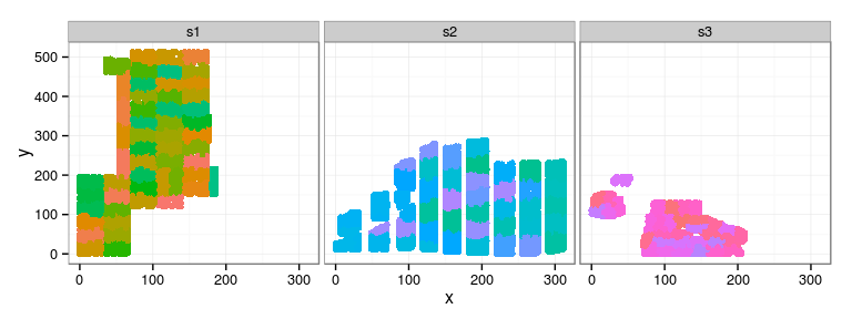
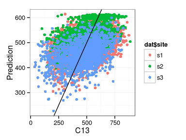
Spatial arrangement
ggplot(douglas, aes(x, y, color = block)) +
  geom_point(show_guide = FALSE) +
  facet_wrap(~ site)
Model fit
Statistical model
Excercise: write the following model in breedR:
\[ \begin{aligned} \mathrm{CR13} = & \mathrm{site} + \mathrm{orig} + fam + bl_\mathrm{site} + fsi + \varepsilon\\ fam \sim & \mathcal{N}(0, \sigma_f^2) \\ bl_s \sim & \mathcal{N}(0, \sigma_{b(s)}^2), \quad s = 1, 2, 3 \\ fsi \sim & \mathcal{N}(0, \sigma_{i}^2) \\ \varepsilon \sim & \mathcal{N}(0, \sigma^2) \end{aligned} \]
- Adjust for blocks within each site
- (possibly with different variabilities)
Preparation of dataset
## create site-wise block variables (i.e. bl_i = bl * Ind(i))
dat <- transform(douglas, bl1 = block, bl2 = block, bl3 = block)
dat$bl1[dat$site != "s1"] <- NA
dat$bl2[dat$site != "s2"] <- NA
dat$bl3[dat$site != "s3"] <- NA
dat <- droplevels(dat)

## variable family (taken as a maternal effect)
dat$fam <- factor(dat$mum)

## family-site interaction variable
dat <- transform(dat, famxsite = factor(fam:site))
Basic Family-Site interaction model
Model with origin and site as fixed effects, and family, blocks and family-site interaction as random effects
reml.tree <- remlf90(fixed  = C13 ~ site + orig,
                     random = ~ fam + bl1 + bl2 + bl3 + famxsite,
                     data = dat, method = 'ai')
Model summary
Linear Mixed Model with pedigree and spatial effects fit by AI-REMLF90 ver. 1.110
   Data: dat
    AIC    BIC logLik
 109427 109470 -54708

Parameters of special components:


Variance components:
         Estimated variances   S.E.
fam                  1339.70 235.07
bl1                   736.37 182.76
bl2                    66.46  50.84
bl3                  1233.80 385.47
famxsite              118.43  61.54
Residual            13653.00 211.56

Fixed effects:
           value    s.e.
site.s1 503.4873  7.4887
site.s2 550.2785  6.7923
site.s3 474.9609  9.6581
orig.pA  -8.9503  4.4835
orig.pB   0.0000  0.0000
orig.pC -42.4425  9.4899
orig.pD  52.2017 44.8236
orig.pE -26.2352 18.7055
orig.pF -37.0728 11.3151
orig.pG -47.1587 23.2942
orig.pH -14.7085 26.4218
orig.pI -49.8486 29.8747
orig.pJ -57.2313 26.3383
orig.pK -53.7943 28.7336
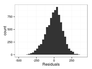
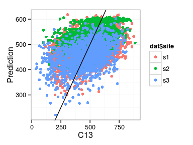
Minimal model diagnosis
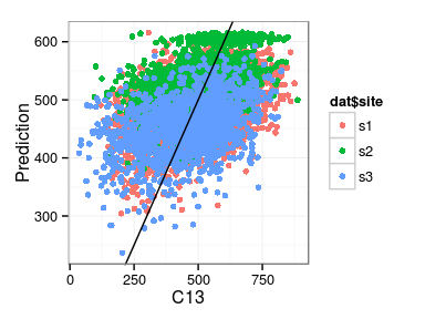
Excercise: produce the following plots:
- histogram of residuals
- fitted vs. observations

Derivation of results
Type-B correlation
reml.tree$var
         Estimated variances    S.E.
fam                 1339.700 235.070
bl1                  736.370 182.760
bl2                   66.463  50.844
bl3                 1233.800 385.470
famxsite             118.430  61.543
Residual           13653.000 211.560
with(reml.tree,
     var['fam', 1] / (var['fam', 1] + var['famxsite', 1])) %>%
  round(2)
[1] 0.92
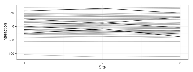
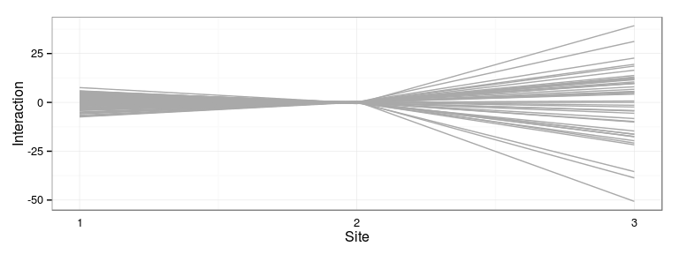
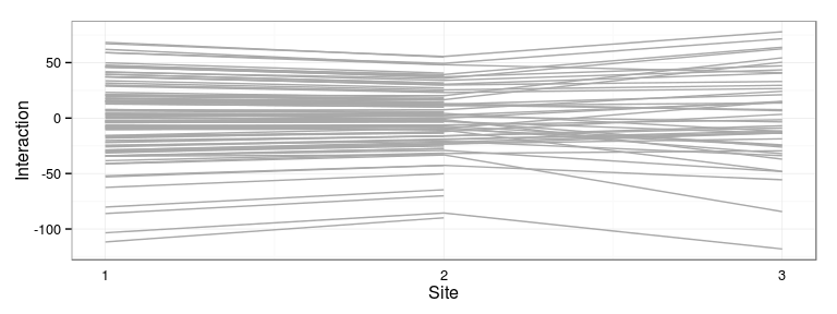
Interaction effect
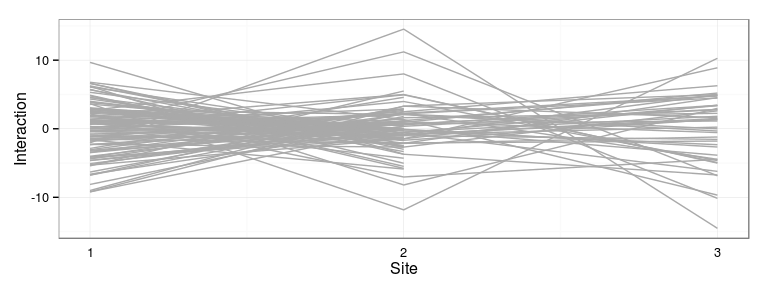
Excercise: produce the following interaction plot:
- predicted family-site interaction by site
- connect values for the same family with a line
Ecovalence
Consider only families present in all the 3 sites
famxsite.tbl <- table(dat$fam, dat$site)
fam3.idx <- apply(famxsite.tbl, 1, function(x) all(x>0))
table(fam3.idx)
fam3.idx
FALSE  TRUE
   64    45
Compute ecovalence by family
Sum of squares by family (across sites) divided by total sum of squares
- (a bit of data-wrangling using
dplyr)
(dat.ecov <-
  dat.fsi %>%
  group_by(fam) %>%
  summarise(ssfam =
              sum(pred_fsi**2)) %>%
  filter(fam3.idx) %>%
  mutate(fratio = ssfam / sum(ssfam)))

## Check
stopifnot(
  all.equal(sum(dat.ecov$fratio), 1)
)
Source: local data frame [45 x 3]

   fam      ssfam      fratio
1    1  18.447072 0.006589986
2    2   8.286972 0.002960417
3    3  58.993908 0.021074836
4    4 109.377567 0.039073769
5    5   4.886922 0.001745792
6    7  20.096726 0.007179304
7    8  33.322147 0.011903920
8    9  10.683869 0.003816679
9   10  18.413615 0.006578034
10  11  67.250109 0.024024261
.. ...        ...         ...
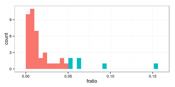
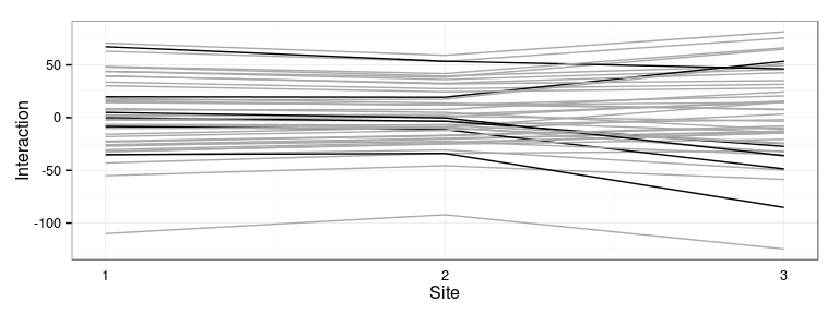
Determine most interactive families
threshold <- 0.05
dat.ecov$hi <- dat.ecov$fratio > threshold
ggplot(dat.ecov, aes(fratio, fill = hi)) +
  geom_histogram(show_guide = FALSE)
Most interactive families: 24 28 38 48 105 106
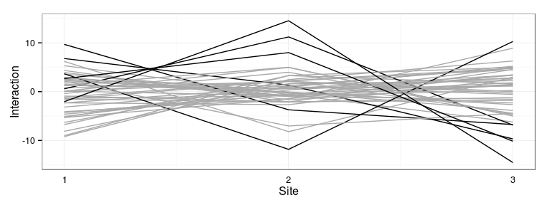
Plot most interactive families
Represent the families which interact the most with the sites:
Correlations of genetic effects across sites
Compute total genetic value
The predicted genetic effect is the sum of the family effect and the family-site interaction (Excercise).
Reshape data
## reshape the genetic values
## by family

(dat.gen <-

   dat.fsi %>%

   select(fam, site, pred_gen) %>%

   tidyr::spread(site, pred_gen) %>%

   tbl_df()
)
Source: local data frame [109 x 4]

   fam          s1         s2         s3
1    1   0.7708066   4.629670   6.755107
2    2 -54.7085993 -55.876654 -55.599421
3    3 -27.5767262 -17.541736 -19.202094
4    4  18.6370661  22.462160  32.831870
5    5  -9.5945562  -9.072929  -6.714122
6    6 -36.1778425 -31.010280         NA
7    7  44.9607625  39.364452  42.434652
8    8  41.1998076  44.446619  48.712357
9    9  40.6242870  36.905050  39.053858
10  10  14.6311835  10.742742   8.711473
.. ...         ...        ...        ...
Compute correlations
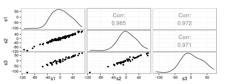
Rank correlations
Kendall (top) and Spearman (bottom)
s1 s2 s3 s1 1.000 0.875 0.834 s2 0.970 1.000 0.851 s3 0.951 0.959 1.000
Prototype zone
site-specific interaction variance?
- The model forced one single variance for the three sites.
- Should we allow different variances?
Statistical model
- Independent site-wise family effects
- Analogous to the blocks effects
\[ \begin{aligned} \mathrm{CR13} = & \mathrm{site} + \mathrm{orig} + fam + bl_\mathrm{site} + f_\mathrm{site} + \varepsilon\\ fam \sim & \mathcal{N}(0, \sigma_f^2) \\ bl_s \sim & \mathcal{N}(0, \sigma_{b(s)}^2), \quad s = 1, 2, 3 \\ f_s \sim & \mathcal{N}(0, \sigma_{f(s)}^2), \quad s = 1, 2, 3 \\ \varepsilon \sim & \mathcal{N}(0, \sigma^2) \end{aligned} \]
Model summary
Things improve a bit wrt the previous model with a single variance. It seems that in site 2 there is not much variation, nor from blocks or for GxE.
Linear Mixed Model with pedigree and spatial effects fit by REMLF90 ver. 1.78
   Data: dat
    AIC     BIC logLik
 109421 unknown -54703

Parameters of special components:


Variance components:
         Estimated variances
fam                 1323.000
bl1                  738.100
bl2                   66.610
bl3                 1237.000
f1                    93.980
f2                     5.789
f3                   662.900
Residual           13630.000

Fixed effects:
           value    s.e.
site.s1 503.3411  7.4347
site.s2 549.4791  6.6367
site.s3 474.4960 10.2681
orig.pA  -8.6398  4.4893
orig.pB   0.0000  0.0000
orig.pC -42.1887  9.3639
orig.pD  52.3152 44.3471
orig.pE -25.6809 18.4917
orig.pF -37.6245 11.2208
orig.pG -37.9558 22.4106
orig.pH  10.1126 25.9501
orig.pI -40.8323 29.5035
orig.pJ -48.0630 26.0029
orig.pK -49.6943 36.9587
Minimal model diagnosis

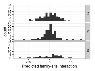
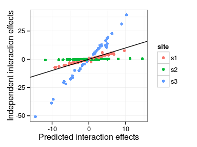
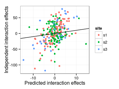
Predicted interaction effects
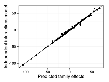
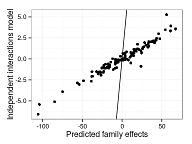
Differences in model predictions
- Main family and interaction effects
- Independent interactions model vs. Single interaction effect
Correlations
Full genetic effect
Correlated effects
Statistical model
The most effective way is to introduce the (expected) correlation between interaction effects across sites into a model parameter.
Among other things, this allows us to predict the genetic value of a family in a site where it was not observed.
\[ \begin{aligned} \mathrm{CR13} = & \mathrm{site} + \mathrm{orig} + fam + bl_\mathrm{site} + fsi + \varepsilon\\ fam \sim & \mathcal{N}(0, \sigma_f^2) \\ bl_s \sim & \mathcal{N}(0, \sigma_{b(s)}^2), \quad s = 1, 2, 3 \\ fsi = \begin{pmatrix} f_1 \\ f_2 \\ f_3 \end{pmatrix} \sim & \mathcal{N}(0, \Sigma_i \otimes \mathrm{I}) \\ \varepsilon \sim & \mathcal{N}(0, \sigma^2) \end{aligned} \]
Model summary
Linear Mixed Model with pedigree and spatial effects fit by REMLF90 ver. 1.78
   Data: dat
    AIC     BIC logLik
 109022 unknown -54500

Parameters of special components:


Variance components:
$fam
[1] 74.67

$bl1
[1] 737.6

$bl2
[1] 67.36

$bl3
[1] 1238

$fsi
     f1   f2   f3
f1 1538 1239 1480
f2 1239 1009 1277
f3 1480 1277 2194

$Residual
[1] 13630


Fixed effects:
            value    s.e.
site.s1 464.26362 10.1012
site.s2 510.67612  9.1863
site.s3 435.08511 12.1330
orig.pA  30.80217 10.8268
orig.pB  38.62992 10.9585
orig.pC  -3.97525 11.3365
orig.pD  91.39946 46.9925
orig.pE  21.13727 20.4114
orig.pF   0.00000  0.0000
orig.pG  10.58885 21.5913
orig.pH  59.81861 24.5012
orig.pI   6.00987 27.6507
orig.pJ   0.37163 24.6342
orig.pK  -3.75109 38.3734
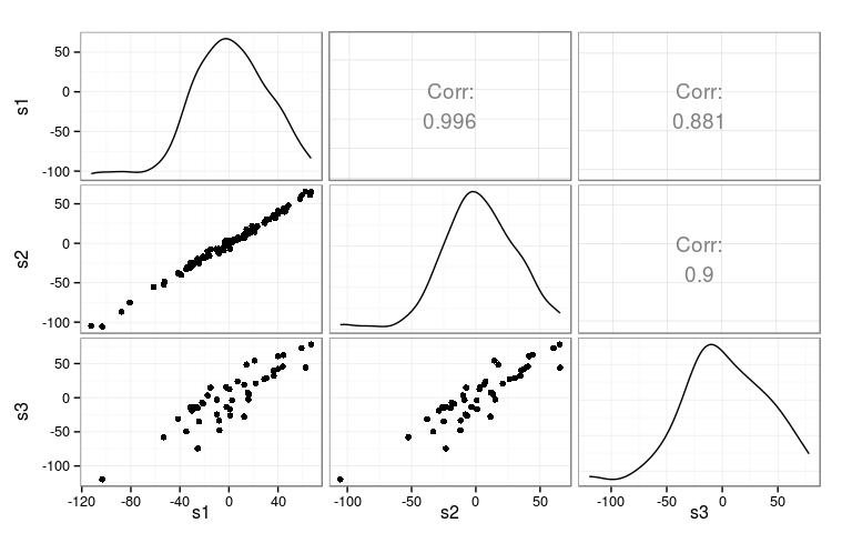
     [,1] [,2] [,3]
[1,] 1.00 0.99 0.81
[2,] 0.99 1.00 0.86
[3,] 0.81 0.86 1.00
Minimal model diagnosis
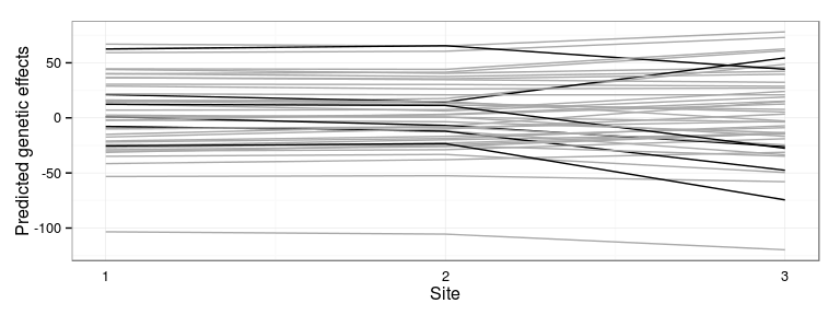
Predicted interaction effects
Differences in predictions
- Main family and interaction effects
- Correlated interactions model vs. Single interaction effect
Correlations

Full genetic effect
- i.e. sum of main and interaction effects
- by family and site
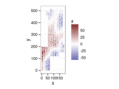
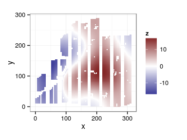
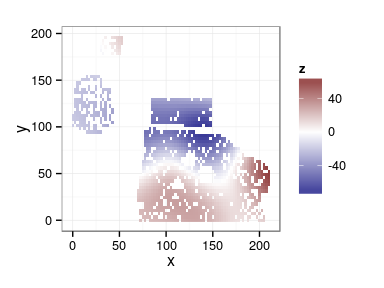
Spatial splines model on each site
Model hack
## Use breedR internal functions to compute splines models on each site
sp1 <- breedR:::breedr_splines(dat[dat$site == 's1', c('x', 'y')])
sp2 <- breedR:::breedr_splines(dat[dat$site == 's2' & !is.na(dat$x) & !is.na(dat$y), c('x', 'y')])
sp3 <- breedR:::breedr_splines(dat[dat$site == 's3', c('x', 'y')])

## Manually build the full incidence matrices with 0
## and the values computed before
mm1 <- model.matrix(sp1)
inc.sp1 <- Matrix::Matrix(0, nrow = nrow(dat), ncol = ncol(mm1))
inc.sp1[dat$site == 's1', ] <- mm1

mm2 <- model.matrix(sp2)
inc.sp2 <- Matrix::Matrix(0, nrow = nrow(dat), ncol = ncol(mm2))
inc.sp2[dat$site == 's2' & !is.na(dat$x) & !is.na(dat$y), ] <- mm2

mm3 <- model.matrix(sp3)
inc.sp3 <- Matrix::Matrix(0, nrow = nrow(dat), ncol = ncol(mm3))
inc.sp3[dat$site == 's3', ] <- mm3

reml.spl <- remlf90(fixed  = C13 ~ site + orig,
                     random = ~ fam + famxsite,
                     generic = list(sp1 = list(inc.sp1,
                                               breedR:::get_structure(sp1)),
                                    sp2 = list(inc.sp2,
                                               breedR:::get_structure(sp2)),
                                    sp3 = list(inc.sp3,
                                               breedR:::get_structure(sp3))),
                     data = dat,
                     method = 'em')
Spatial effects by site